
Bond Return Components
This section shows that a security’s total return consists of an income component and a price change component. It introduces a few other concepts specific to bonds, and then shows how those two return components contribute to bond returns in a varying manner over nearly a century. Don’t worry, there’s only one formula involved and you already understand it!
Introduction
- A security’s total return normally consists of two parts, its income return and its price return.
- Price returns attracts most attention because prices changes are frequent and large, whereas income returns over short periods are very small and changes are infrequent. But over longer periods the story reverses.
Bond Price Changes
- A bond is issued and eventually matures at its “par” price of $100 but its price changes in the interim, in the opposite direction as interest rates. This occurs because its original interest payment ("coupons") become inappropriate when interest rates change.
- If interest rates fall, an existing bond’s fixed coupons become more valuable and the bond’s price rises.
- The opposite occurs if interest rates rise: an existing bond’s coupons are no longer as valuable and its price falls.
- A bond’s coupons are fixed but its price is not; a bond’s price constantly adjusts to keep its expected returns in line with current interest rates.
- The longer a bond’s maturity, the greater its sensitivity to interest rate changes.
Yield to Maturity
- It its interim price doesn’t equal par, a bond’s initial interest rate doesn’t accurately measure its expected return.
- A bond’s yield-to-maturity or “yield” accurately measures its expected annual return if held to maturity, and reflects interest payments along with the bond’s expected price movement towards par at maturity.
Results
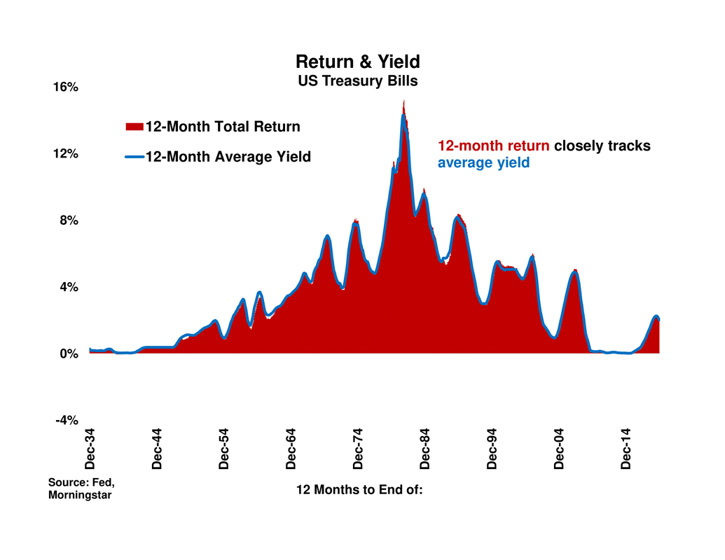
- T-Bill returns over twelve-month periods are almost identical to their average yield over the same twelve months, due their very short maturity (1-2 months) and their resulting price insensitivity to interim yield changes.
- The monthly price returns of the US long government bond index are far more volatile than its income returns.
- For 10-year returns, the situation reverses: even among long-term bonds, which are most price-sensitive to interest rate changes, income returns dominate price returns.
- Negative price returns exert an extensive drag on bond returns from the mid-1950’s until the mid-1980’s. However, the negative impact doesn’t overcome the strong positive impact from income returns, and total returns stay positive throughout.
- Beginning in the 1980’s, positive price returns add to income returns for nearly 40 years.
- Income returns are even more pronounced than price returns in the 10-year returns of intermediate bonds, whose prices are less sensitive to interest rate changes.
- The long-bond index’s 10-year income return is almost identical to its 10-year average yield; bond income returns are very closely tied to bond yields.
- Long bonds’ ten-year price returns reflects the path of long yields. Yields’ long climb from the 1950’s through the 1970’s, along with rising inflation, causes significant negative price returns. Yields peak in late 1981, after Federal Reserve Chairman Paul Volcker begins to wring inflationary pressures out of the US economy, and then fall and thereby boost price and total returns for the next four decades.
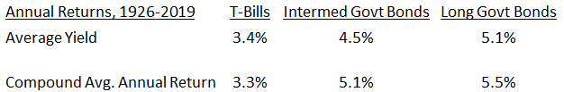
- Over nearly a century, intermediate- and long-government bonds’ higher returns compared to T-Bills are not surprising but instead reflect their higher average yields, which in turn represent compensation for the greater uncertainty inherent in longer bond maturities.
Conclusion
- Price return volatility is very pronounced among monthly returns, but at longer holding periods, income returns – which closely reflect average yields - exert the dominant effect on overall bond returns. The income return even offsets negative price returns from the mid-1950’s to the early 1980’s and keeps total returns positive.
- The four decade decline in yields from their 15% peak in 1981 proves a boon to bondholders. But with yields now only 1.5% and 0.4% for 20-and 5-year government bonds, very little interest income is on tap to provide returns, let alone to buffer investors if bond yields should rise and bond prices fall.
Introduction
The Return Characteristics section introduced the formula for a security’s total return:
Nearly all payments consist of income, either interest income for bonds or dividend income for stocks. We thus rewrite the total return equation as two parts, its income return and its price return:

For example, a security with a starting price of $100 that pays $2 of income in the period and whose price rises to $105 during the period has a total return of 7%, its 2% income return and a 5% price return as shown below:

Showing the two return components separately allows us to better understand the source of bond returns. The price return attracts the lion’s share of attention because prices change by the minute and often quite dramatically, whereas the income return over short periods is very small and barely changes at all. But over longer periods the story reverses.
Bond Price Changes
A bond is typically issued and eventually matures at the same price of $100, also known as its “par” value, but its price on the secondary market changes in the interim as interest rates change. A bond’s price moves in the opposite direction as interest rates: as interest rates fall a bond’s price rises, and vice versa as rates fall. This occurs because a bond’s original interest payments (“coupons”) become inappropriate, relative to those of newly-issued bonds, when interest rates change.
For example, a bond issued with a fixed 5% annual interest rate pays a $5 coupon each year until maturity, but becomes more valuable if interest rates fall to 4%. The bond’s price is immediately bid upward to the point that its expected subsequent decline, from its new price to par value at maturity, partially offsets its high coupons and lowers its return to 4%, equal to the current fair interest rate. This example is shown in the Details tab.
The opposite occurs if interest rates rise: the bond’s $5 coupons are no longer competitive and its price falls immediately so that its subsequent price rise to par at maturity, along with its $5 coupons, provides a return in line with the new higher interest rate.
The end result is that a bond’s coupons are fixed but its price is not: a bond’s price constantly adjusts to keep its expected returns in line with current interest rates.
Bonds with longer maturities are also more sensitive to interest rate changes than are shorter-maturity bonds. The longer the bond maturity the greater its number of inappropriate coupons, and so the larger its price change must be to offset those coupons. An example is shown in the Details tab.
Yield to Maturity
If its interim price has moved from its initial par value, a bond’s initial interest rate doesn’t reflect the price’s eventual return to par at maturity. Instead, yield-to-maturity or “yield” measures a bond’s effective interest rate, essentially its expected return if held to maturity. A bond’s yield includes both its interest payments and its movement back to par from its current price. If the bond’s price is below par, its yield includes upwards price movement towards par at maturity and if its price is above par, its yield similarly reflects downwards price movement towards par.
Results
In the following discussion, each month’s income return includes interest payments and any price movement towards par as reflected in the month’s starting yield. The price return reflects all other price movement.
|
T-Bill returns over twelve-month periods, in red, are almost identical to their average yield over the same twelve months. T-Bills maturities are very short, only one or two months, and so their price is barely affected by interest rate changes and they essentially “return their yield” in almost every period. We thus restrict the rest of our attention to intermediate- and long-term US federal government bonds, whose longer maturity makes their prices more sensitive to interest rate changes. |
|
|
The monthly income and price returns of the US long government bond index are shown in the first two slides to the right, whose scales are the same to allow comparison. At these short holding periods, price returns in blue completely dominate income returns in red; the monthly income return is barely even visible!
But the story changes completely as the investment holding period lengthens to ten years. The third chart shows the ten-year annualized income return in red and price return in blue, along with the total return (their sum) as the black line, for the long-government bond index. If anything, income returns now dominate price returns! The highly volatile monthly price returns in the first chart often cancel each other over time, whereas positive ongoing interest payments, small as they may first seem, slowly but steadily accumulate and become the most important part of the ten-year bond return. The income return is even more important for the intermediate-term government bonds in the fourth chart, because their prices are less sensitive to interest rate changes than are long-bond prices. |
|
|
The next two charts on the right track long-bond yields and how they translate into income and price returns. The first shows the ten-year income return of the long bond, along with its monthly yield in orange and its ten-year average yield in blue. The ten-year income return is almost identical to its ten-year average yield; bond income returns are very closely tied to bond yields. The second chart shows the long bond’s annualized ten-year price return along with its monthly yield. The multi-decade rise in yields begins innocuously in the 1950’s, then accelerates along with rising inflation in the 1960’s and 1970’s and causes negative price returns during this time. Bond yields peak in late 1981 and then start to decline, after Federal Reserve Chairman Paul Volcker throws the US into two consecutive recessions to wring inflation out of the economy. The next four decades of falling yields, including the Federal Reserve’s responses to the 2008 financial crisis and the 2020 Covid pandemic, generate positive price returns for bondholders. |
|
Armed with the proof that interest rates (“yields”) instead of price changes matter most to bond returns over longer periods, the next table revisits the bond returns from the Stocks & Bonds Return Characteristics section but first shows their average yield at each month end. Viewed in relation to their yields, the higher returns moving from T-Bills to intermediate- and then to long-maturity bonds are not surprising: their returns are higher because their yields are higher!
|
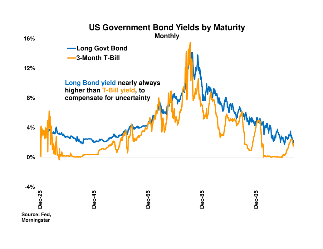
Even made to a high-quality borrower like the US federal government, a twenty-year loan carries more risk of unexpected inflation and non-payment than does a three-month loan; uncertainty increases with a bond’s maturity. Thus as shown in the chart to the right, longer-maturity bonds usually offer higher yields in order to compensate investors for their higher uncertainty. |
|
Conclusion
Despite price returns’ high monthly volatility, income returns – which closely reflect average bond yields - exert the dominant effect on bond total returns at longer holding periods. The income return even offsets negative price returns from the mid-1950’s to the early 1980’s; not once does the total return become negative for intermediate or long bonds. The four-decade decline in yields from their 15% peak in 1981 and the commensurate boost to bond prices prove a boon to bondholders, but somewhat ominously, income returns also gradually decline along with lower yields. With yields at the start of 2021 merely 1.5% and 0.4% for 20-and 5-year government bonds, there’s very little interest income on tap to provide returns, let alone to buffer investors if bond yields should rise and bond prices fall.
1) Example of Bond Price Changes
We use the Main section’s example of a 5% coupon 5-year government bond and assume that the day after issuance, the fair interest rate for such a bond falls to 4%. Although government bond coupons are paid semi-annually, for simplicity we instead show them paid annually.
Also, bonds are issued in $1000 denominations but their prices are quoted per hundred dollars of par. For example, a bond is said to be trading at $95 when its price is actually $950, or $95 per hundred dollars of its par value of $1000. For simplicity, we treat the bond as though its true par value is $100.
Also to simplify the tables, we show the bond’s final price as $100, instead of as zero with a principal repayment of $100. Finally, the example assumes that the marginal buyer or seller of bonds holds them in a tax-free account for which capital gains or losses are treated the same as interest income.
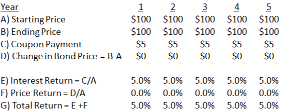
The first table shows the situation when the bond is first issued with a $5 coupon, representing a 5% interest rate, and the interest rate never changes. Its price stays at $100 each year and its $5 coupon thereby represents a 5% return on each year’s starting price.
We use the Main section’s example of a 5% coupon 5-year government bond and assume that the day after issuance, the fair interest rate for such a bond falls to 4%. Although government bond coupons are paid semi-annually, for simplicity we instead show them paid annually.
Also, bonds are issued in $1000 denominations but their prices are quoted per hundred dollars of par. For example, a bond is said to be trading at $95 when its price is actually $950, or $95 per hundred dollars of its par value of $1000. For simplicity, we treat the bond as though its true par value is $100.
Also to simplify the tables, we show the bond’s final price as $100, instead of as zero with a principal repayment of $100. Finally, the example assumes that the marginal buyer or seller of bonds holds them in a tax-free account for which capital gains or losses are treated the same as interest income.
The first table shows the situation when the bond is first issued with a $5 coupon, representing a 5% interest rate, and the interest rate never changes. Its price stays at $100 each year and its $5 coupon thereby represents a 5% return on each year’s starting price.
The next table shows what happens if interest rates fall to 4% the day after the bond’s issue and doesn't change thereafter. Its price gets bid upwards in the secondary market because both buyers and sellers realize that its $5 coupons are more valuable in a 4% interest rate environment. Its price is bid up to $104.45, from which point it is then expected to decline towards its par value of $100 over the next five years. The expected price decline coupled with its $5 annual coupon together create a 4% annual return, which puts the bond on an equal footing with newly-issued bonds that reflect a 4% interest rate.
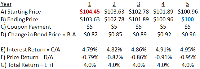
At any price higher than $104.45, the bond’s expected return is less than 4% per year and so investors won’t want to hold it and will sell it until its price equals $104.45. At any price lower than $104.45, the bond’s expected return is higher than 4% and so investors will want to own it and will buy it until its price increases to $104.45.
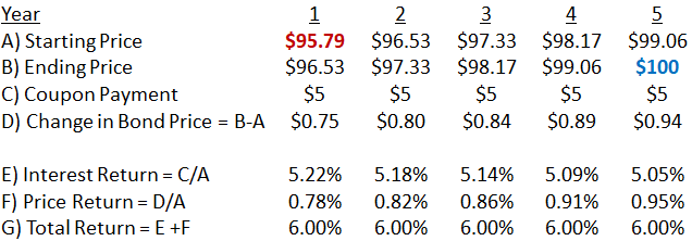
The next table shows what happens when the opposite occurs and interest rates rise to 6% from their initial 5%. The bond's price falls because buyers and sellers all recognize that its $5 coupons are less valuable in a 6% interest rate environment. Its price declines to $95.79, and is expected thereafter to rise towards its par value of $100 over the next five years. The expected price rise and the bond's $5 annual coupon combine for a 6% annual return, leaving the bond fairly priced compared to newly-issued bonds with a 6% interest rate.
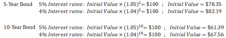
2) When 5% interest rates fall to 4% in the prior example, the 5-year bond price rises by 4.45% to $104.45. The table below show what occurs in the the same situation for a 10-year bond.
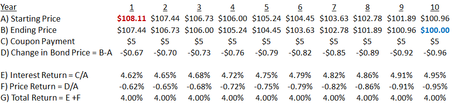
The 10-year bond’s price rises from $100 to $108.11, an increase of 8.11%, slightly less than double the 5-year bond’s increase. The longer-maturity bond’s price rises more because it has many more fixed-amount coupons, which are more valuable in the new, lower-rate environment.
The same occurs in reverse if interest rates rise: the longer the bond’s maturity, the greater the number of coupons which are less valuable in the new, higher interest rate environment, and so the larger the bond’s price decline. Regardless of the direction of the interest rate change, the resulting bond price change is larger for a bond of longer maturity.
The same occurs in reverse if interest rates rise: the longer the bond’s maturity, the greater the number of coupons which are less valuable in the new, higher interest rate environment, and so the larger the bond’s price decline. Regardless of the direction of the interest rate change, the resulting bond price change is larger for a bond of longer maturity.
3a) In the prior examples, after its initial change the interest rate then stayed constant until the bond’s maturity. In reality, interest rates change numerous times between a bond’s issuance and maturity dates. Even though interest rates will change, the above framework retains its ability to properly assign a bond’s value immediately after the most recent interest rate change . The model is then updated with each successive interest rate change.
3b) In the prior examples we wrote that a change in interest rates affects a bond’s price through its effect on the attractiveness of an existing bond’s coupons. This is often the simplest way to remember that bond prices and interest rates are inversely related.
But the current value of a bond’s principal repayment at maturity, not just its coupons, is also inversely related to interest rate changes. For example, what’s the value at the issuance date of a 5-year bond’s $100 principal repayment, if interest rates are 5%? Its value is the amount one must invest now so that at a 5% compounded annual return, it will be worth $100 in five years. We plug in the interest rate, number of years and ending value into the compound return formula below, to solve for the initial value.
But the current value of a bond’s principal repayment at maturity, not just its coupons, is also inversely related to interest rate changes. For example, what’s the value at the issuance date of a 5-year bond’s $100 principal repayment, if interest rates are 5%? Its value is the amount one must invest now so that at a 5% compounded annual return, it will be worth $100 in five years. We plug in the interest rate, number of years and ending value into the compound return formula below, to solve for the initial value.


The initial value of the bond’s principal payment is $78.35.
What happens if interest rates fall to 4%? The principal repayment's initial value increases to $82.19, as shown below.
What happens if interest rates fall to 4%? The principal repayment's initial value increases to $82.19, as shown below.

If interest rates instead rise to 6%, the principal repayment’s initial value declines to $74.73, as shown below.

So we see that a bond principal repayment’s value is inversely related to interest rate changes. The intuition is that the higher the interest rate, the smaller the up-front investment required to receive the fixed principal repayment upon the bond’s maturity.
3c) In part 2 we wrote that a longer-maturity bond’s price is more sensitive to interest rate changes because it has more coupons than a shorter-maturity bond. But the number of coupons isn’t the only difference between the two bonds: the difference in maturity also matters.
For example, consider a 5-year and a 10-year bond. Both make a $100 principal repayment upon maturity. Using the compound return formula from part 3b, what’s the change in the initial value of the bonds’ principal when interest rates change from 5% to 4%?
For example, consider a 5-year and a 10-year bond. Both make a $100 principal repayment upon maturity. Using the compound return formula from part 3b, what’s the change in the initial value of the bonds’ principal when interest rates change from 5% to 4%?
The percentage change is much larger for the 10-year bond, 10% of its initial value versus only 4.9% for the 5-year bond. Thus longer-maturity bonds are more sensitive to interest rate changes than are shorter-maturity bonds. The intuition is that a given interest rate change “ripples through” many more years and thereby induces a larger percentage change in the up-front investment needed to receive the principal repayment upon maturity, for a longer- than for a shorter-maturity bond.
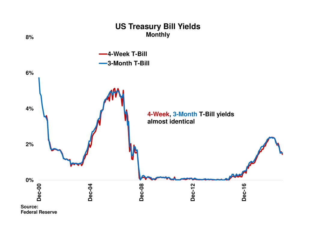
4a) The primary data source of bond returns and yields in this section is the Ibbotson SBBI Yearbook (“Stocks, Bonds, Bills, and Inflation”). Its T-Bill, intermediate- and long-government bond returns all begin in January 1926. However, the SBBI Yearbook doesn’t provide T-Bill yields, whereas it provides monthly yields for the other two government bond types.
|
As a proxy for the SBBI T-Bill series, which is “the shortest term bill having not less than one month to maturity”, we instead use the 3-Month T-Bill yield from the US Federal Reserve (“the Fed”). The chart to the right compares the Fed’s 3-Month T-Bill yield to its 4-Week T-Bill yield since both have been available, and the two are nearly identical. |
|
The Fed’s 3-Month T-Bill yield starts in 1934 and covers most of the same historical period as SBBI, and we use this series’ yield in the chart in the Main tab which compares twelve-month T-Bill returns to the average yield over the same twelve months.
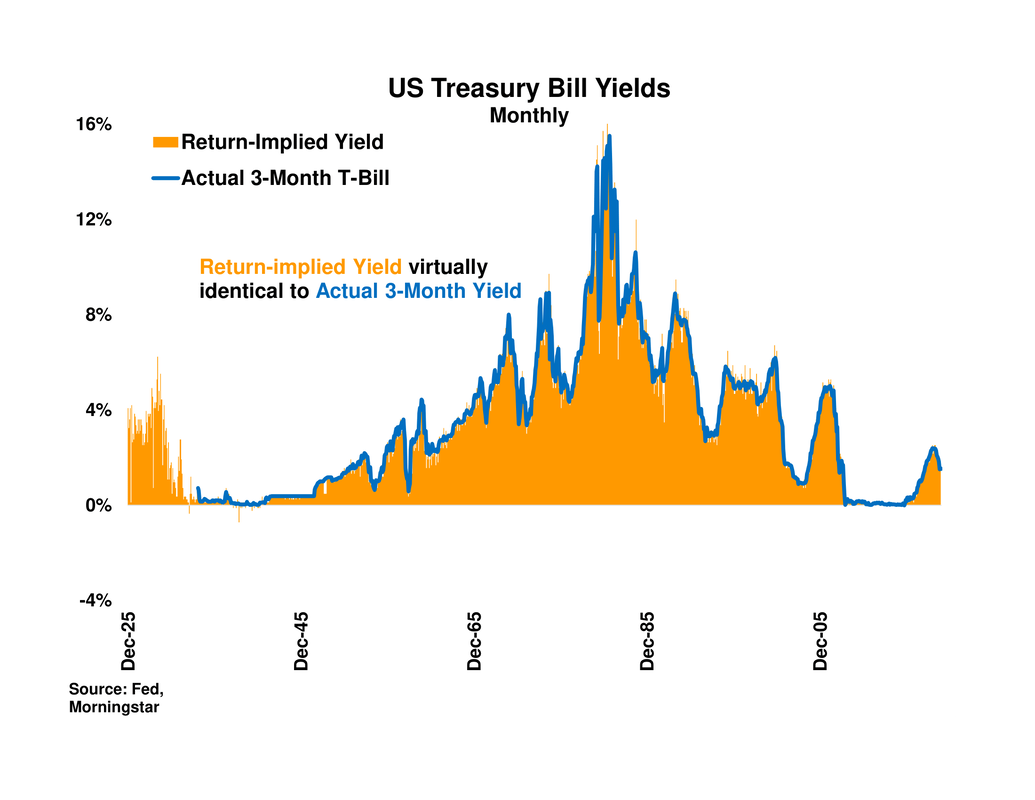
4b) The Fed’s 3-Month T-Bill series mentioned in point 3a begins only in 1934, which leaves a gap of yields (but not returns) from December 1925 to 1933. To deal with the missing yields, we first create a series of synthetic T-Bill yields from their monthly returns. Each month’s ending synthetic yield is simply the next month’s T-Bill return, annualized by multiplying the return by twelve
|
The chart to the right compares the synthetic “return-implied” T-bill yield to the Fed’s 3-Month T-Bill yield from 1934 onward, and the two are virtually identical. |
|
The table of average returns and yields from 1926-2019 in the Main tab, and the chart which follows it and compares T-Bill to Long-Government Bond yields, both use the synthetic “return-implied” yield from December 1925 to December 1933 and thereafter use the Fed’s 3-Month T-Bill yield.